Sparse matrix computations are essential in several machine learning and scientific applications. Most elements in a sparse matrix are zero, so the matrix is stored in compressed form to skip computations on zeros. The compression makes sparse methods irregular, challenging efficient use of a processor's memory subsystem. In this post, I explain why a new definition of regularity is needed to improve the performance of sparse codes.
What does regularity mean?
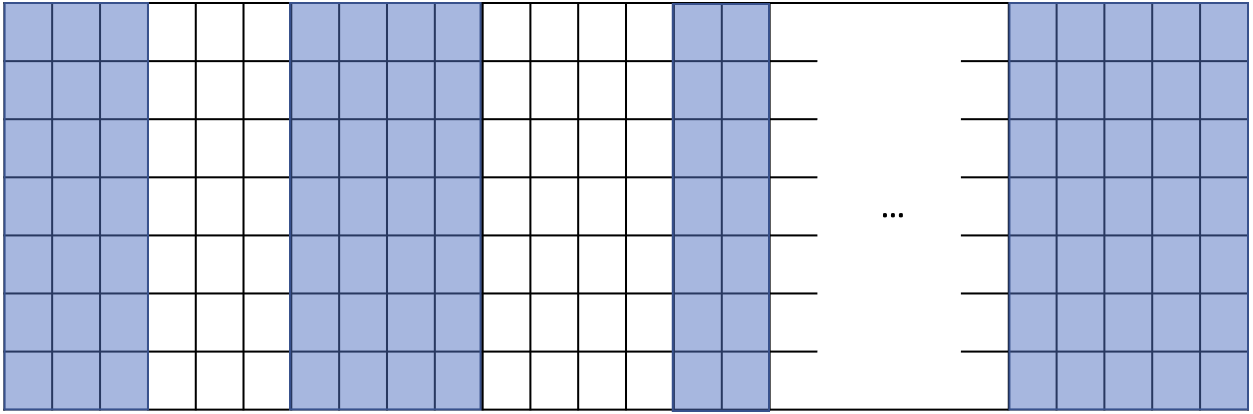
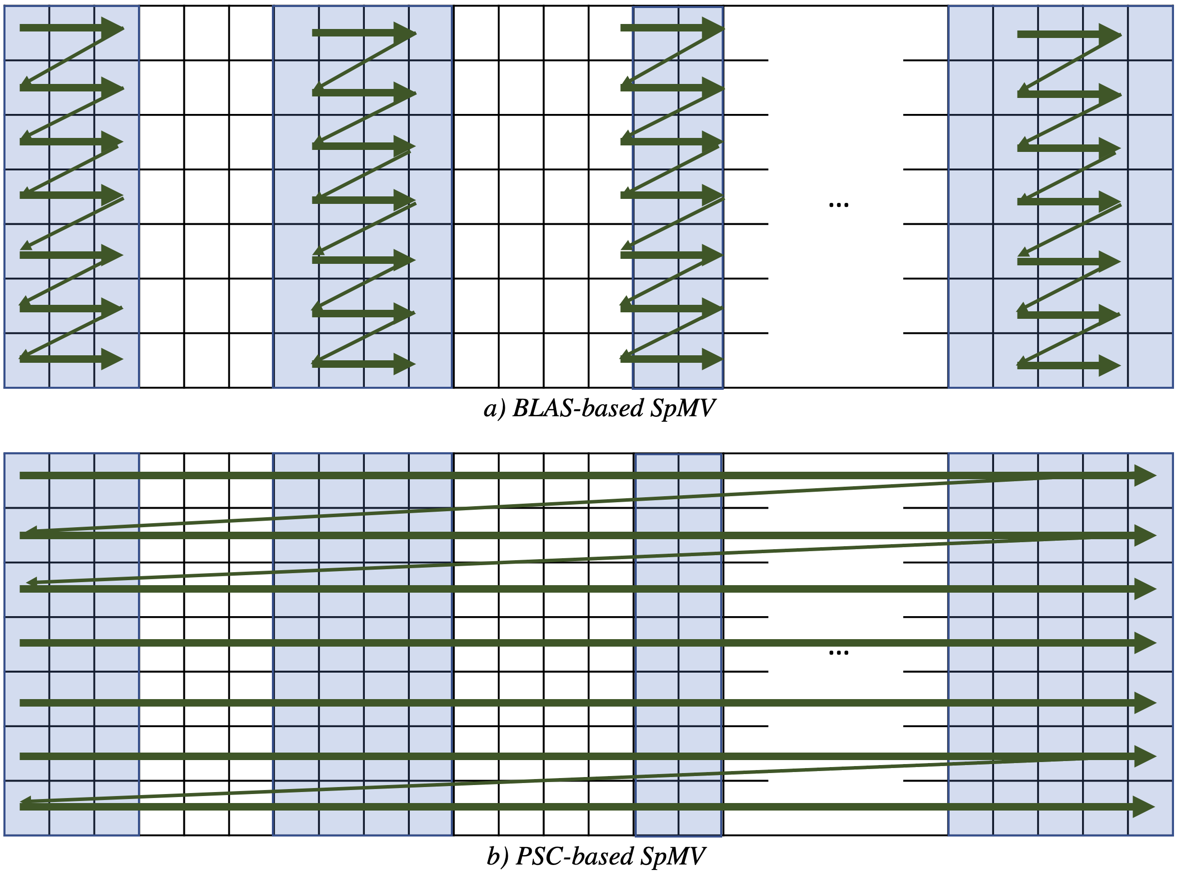
A common approach to accelerate a sparse method is to break it into small “regular” computations, i.e., computations that can use machine resources efficiently. Let’s use the example shown in Figure 1 to explain the current definition of regularity and its pitfalls. The matrix in Figure 1 illustrates a sparse matrix, where rectangular blocks are dense submatrices containing nonzero elements. How would you find regularity in the shown matrix? Probably, most people see each rectangle as a regular region. Not surprisingly, practitioners and researchers typically use the same technique. They find dense submatrices in the sparse matrix and then use efficient dense matrix routines, e.g., a BLAS implementation, to perform the computation. However, this is not the most efficient implementation because it neglects the contiguous storage of nonzero elements in a compressed matrix format. Let’s see how regular regions should be re-defined for sparse code with an example.
Why should we redefine regularity?
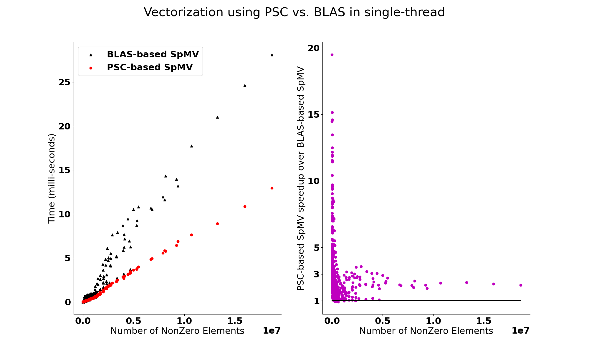
Compressed storage formats in sparse code lead to random accesses. Removing random accesses in dense matrices is often possible by building new schedules and/or code rewriting. This makes prior definitions of regular codes, such as BLAS, heavily rely on strided accesses. But avoiding random accesses in sparse codes is impossible or leads to inefficient execution. There is room for performance optimization even with some random accesses, which demands a new definition of regularity. This new definition is called partially strided codelets . Partially strided codelets can express any regularity in a computation region and provide a qualitative and quantitative measure to apply performance optimization techniques to sparse methods. For example, if a computational region can not be expressed with a PSC, there is no performance benefit in vectorizing it with the given storage. Since sparse methods are memory-bound, PSCs are vital to exploit the memory sub-system in current architectures.
							 for (int i = 0; i < m; ++i)
							 	for (int j = Ap[i]; j < Ap[i+1]; ++j)
							 		y[i] += Ax[j] * x[Ai[j]];
What are PSCs?
We model accesses within a computation region with access functions. An access function maps an iteration space to a data space. When there is at least one strided access function and one random (unstrided) access function, the region is defined as a PSC. If all access functions are strided, then it is a fully strided region, e.g. a BLAS call. Finding PSCs can be done at compile-time or runtime. For example, the SpMV code shown in Listing 1 is a PSC. However, for efficiency, we should use sparsity information to extract smaller and more performant PSCs. We have used a differentiation-based PSC synthesis along with a graph-covering problem to find PSCs in SpMV, sparse triangular solver, and sparse-dense matrix multiplication. Please check our paper and code repository for more details.