Loop statements are fundamental in any program and take most of the execution time. If iterations of a loop are independent, then they can run in parallel thus the loop is called a parallel loop. If iterations of a loop require a specific order of execution for correctness, then the loop is called a loop-carried dependence. Parallel loops provide an easier way to use all parallel resources, so algorithms are designed or redesigned to use parallel loops for better performance. I use matrix operations in this post to illustrate the performance gap between a parallel loop and a loop-carried dependence and discuss how sparse data bridges the gap.
Background
I use two popular matrix operations, matrix-vector multiplication (MV) and lower triangular solve (SV), to compare the performance of a loop-carried dependence with a parallel loop. The outermost loop of MV is parallel, and the outermost loop of SV carries dependence. Figure 1 shows the code for the two operations. The two operations can be applied to a sparse matrix, a matrix in which most of its elements are zeros. The operation’s code and the matrix storage format should change to skip instructions corresponding to zero elements. This zero skipping also removes some dependent iterations in the SV, improving its parallel execution. I use these two operations as a case study to discuss the performance of parallel loops and loop-carried dependence.
							 /// Computing b=A*x
							 for(int i = 0; i < M; i++)
							    for(int j = 0; j < N; j++)
							       b[i] += A[i][j] * x[j];

							 /// Solving Lx=b for x
							 for(int i = 0; i < M; i++) {
							    for(int j = 0; j < i; j++)
							       x[i] -= L[i][j] * x[j];
							    x[i] /= L[i][i];
							 }
The effect of sparse dependence
Figure 2 compares the performance of SV and MV operations when the input is dense and sparse matrices on 40 Intel Skylake cores (dual socket). Dense matrices are randomly generated, and sparse matrices are the lower triangular part of all symmetric positive definite matrices larger than 1 million nonzero elements from SuiteSparse. For dense operations, MKL (Math Kernel Library) BLAS (Basic Linear Algebra Subroutine) calls to GEMV, and TRSM are used. For sparse operations, two different implementations are selected, MKL (I/E) and Sympiler. MKL benefits from vector and thread-level parallelism, and Sympiler uses thread-level parallelism (scalarized). The theoretical FLOP (floating-point operation) of the matrix operation is used to compute the GFLIP/s in different implementations. The performance gap between SV and MV operations is different for sparse and dense matrices.
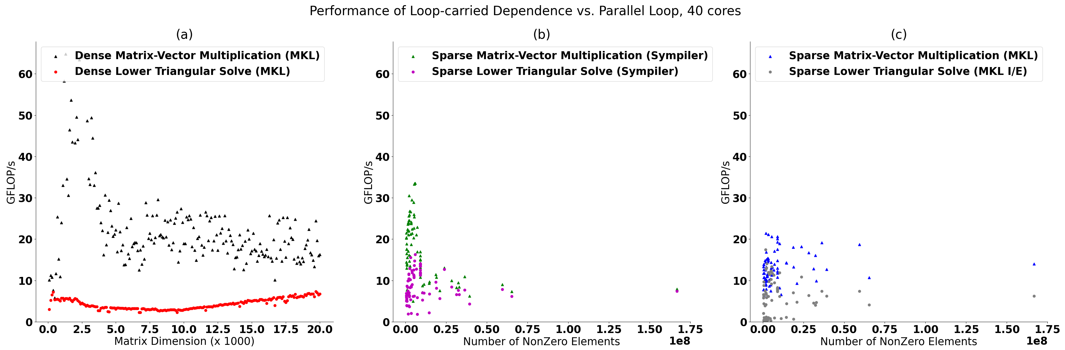
The performance MV and SV for sparse matrices are shown in Figures 2b and 2c for two different implementations. The geometric mean speedups of sparse MV over sparse SV for Sympiler and MKL are 2X and 3.3X, respectively. As shown, compared to the dense implementation, the gap is reduced noticeably (from 5.2X to 2X). The performance of Sympiler sparse MV is between 5-33 GFLOP/s, and the performance of Sympiler sparse SV is between 2-16 GFLOPS/s, which are close to each other. The main reason is dependence removal due to zero elements in the matrix. This reduced gap can potentially help pre-conditioned iterative solvers, which have a fast convergence rate, but computing the preconditioner often becomes their bottleneck and thus makes them slower than other iterative solvers that rely on parallel loops. Note that dense and sparse matrices are not equivalent, and their performance cannot be compared one-to-one. However, when the number of nonzero elements is identical, the performance numbers provide insight. The code repository, including setup details, data, and scripts, for the experiment, is available here.
Limitations
Parallelism in loop-carried sparse dependence comes from properties of sparse data and it has some limitations. Extracting parallelism requires a pre-processing phase, a runtime inspection, that creates an overhead. Since the computation pattern remains static and known at compile-time in many applications, the inspection is done once and reused multiple times, amortizing the cost over the number of runs. For example, in iterative solvers, the preconditioner determines the sparsity of the SV operation which is used in all iterations of the solver. Also, since parallelism is data-dependent, the performance gap can increase when the computation pattern is inherently sequential, i.e., no thread-level parallelism. However, there are sparsification techniques to alleviate this problem.